# Lab 3 翻译
Assigned: Wednesday, Mar 17, 2021 Due: Tuesday, Apr 6, 2021
In this lab, you will implement a query optimizer on top of SimpleDB. The main tasks include implementing a selectivity estimation framework and a cost-based optimizer. You have freedom as to exactly what you implement, but we recommend using something similar to the Selinger cost-based optimizer discussed in class (Lecture 9).
在这个实室中,你将在SimpleDB之上实现一个查询优化器。主要任务包括实现一个选择性估计框架和一个基于成本的优化器。你可以自由选择具体的实现方式,但我们建议使用类似于课堂上讨论的Selinger基于成本的优化器(第9讲)。
The remainder of this document describes what is involved in adding optimizer support and provides a basic outline of how you do so.
本文件的其余部分描述了添加优化器支持所涉及的内容,并提供了一个关于如何添加优化器的基本概要。
As with the previous lab, we recommend that you start as early as possible.
与前一个实室一样,我们建议你尽可能早地开始。
# 1. Getting started
You should begin with the code you submitted for Lab 2. (If you did not submit code for Lab 2, or your solution didn't work properly, contact us to discuss options.)
你应该从你为实室2提交的代码开始。(如果你没有为实室2提交代码,或者你的解决方案没有正常工作,请与我们联系,讨论各种方案。)
We have provided you with extra test cases as well as source code files for this lab that are not in the original code distribution you received. We again encourage you to develop your own test suite in addition to the ones we have provided.
我们为这个实室提供了额外的测试案例以及源代码文件,这些文件不在你收到的原始代码分发中。我们再次鼓励你在我们提供的测试案例之外,开发你自己的测试套件。
You will need to add these new files to your release. The easiest way to do this is to change to your project directory (probably called simple-db-hw) and pull from the master GitHub repository:
你将需要把这些新文件添加到你的版本中。最简单的方法是换到你的项目目录(可能叫simple-db-hw),然后从GitHub的主仓库拉出。
$ cd simple-db-hw $ git pull upstream master
# 1.1. Implementation hints
We suggest exercises along this document to guide your implementation, but you may find that a different order makes more sense for you. As before, we will grade your assignment by looking at your code and verifying that you have passed the test for the ant targets test and systemtest. See Section 3.4 for a complete discussion of grading and the tests you will need to pass.
我们建议沿着这份文件进行练习,以指导你的实施,但你可能会发现不同的顺序对你更有意义。和以前一样,我们将通过查看你的代码并验证你是否通过了蚂蚁目标测试和systemtest的测试来给你的作业评分。关于评分和你需要通过的测试的完整讨论见第3.4节。
Here's a rough outline of one way you might proceed with this lab. More details on these steps are given in Section 2 below.
下面是你可能进行这个实验的一个粗略大纲。关于这些步骤的更多细节将在下文第2节给出。
Implement the methods in the TableStats class that allow it to estimate selectivities of filters and cost of scans, using histograms (skeleton provided for the IntHistogram class) or some other form of statistics of your devising.
实现TableStats类中的方法,使其能够使用直方图(IntHistogram类提供的骨架)或你设计的其他形式的统计数据来估计过滤器的选择性和扫描的成本。
Implement the methods in the JoinOptimizer class that allow it to estimate the cost and selectivities of joins.
实现JoinOptimizer类中的方法,使其能够估计 join 的成本和选择性。
Write the orderJoins method in JoinOptimizer. This method must produce an optimal ordering for a series of joins (likely using the Selinger algorithm), given statistics computed in the previous two steps.
编写JoinOptimizer中的orderJoins方法。这个方法必须为一系列的连接产生一个最佳的顺序(可能使用Selinger算法),给定前两个步骤中计算的统计数据。
# 2. Optimizer outline
Recall that the main idea of a cost-based optimizer is to:
回顾一下,基于成本的优化器的主要思想是:
Use statistics about tables to estimate "costs" of different query plans. Typically, the cost of a plan is related to the cardinalities of (number of tuples produced by) intermediate joins and selections, as well as the selectivity of filter and join predicates.
使用关于表的统计数据来估计不同查询计划的 "成本"。通常情况下,一个计划的成本与中间连接和选择的cardinalities(产生的 tuple 数量),以及过滤器和连接谓词的选择性有关。
Use these statistics to order joins and selections in an optimal way, and to select the best implementation for join algorithms from amongst several alternatives. In this lab, you will implement code to perform both of these functions.
利用这些统计数据,以最佳方式排列连接和选择,并从几个备选方案中选择连接算法的最佳实现。 在本实室中,你将实现代码以执行这两项功能。
The optimizer will be invoked from simpledb/Parser.java. You may wish to review the lab 2 parser exercise before starting this lab. Briefly, if you have a catalog file catalog.txt describing your tables, you can run the parser by typing:
优化器将从simpledb/Parser.java调用。在开始这个实验之前,你可能希望回顾一下实验2的解析器练习。简而言之,如果你有一个描述你的表的目录文件catalog.txt,你可以通过输入来运行解析器。
java -jar dist/simpledb.jar parser catalog.txt
When the Parser is invoked, it will compute statistics over all of the tables (using statistics code you provide). When a query is issued, the parser will convert the query into a logical plan representation and then call your query optimizer to generate an optimal plan.
当解析器被调用时,它将对所有的表进行统计计算(使用你提供的统计代码)。当一个查询被发出时,解析器将把查询转换成逻辑计划表示,然后调用你的查询优化器来生成一个最佳计划。
# 2.1 Overall Optimizer Structure
Before getting started with the implementation, you need to understand the overall structure of the SimpleDB optimizer. The overall control flow of the SimpleDB modules of the parser and optimizer is shown in Figure 1.
在开始实施之前,你需要了解SimpleDB优化器的整体结构。分析器和优化器的SimpleDB模块的整体控制流程如图1所示。
 Figure 1: Diagram illustrating classes, methods, and objects used in the parser
图1:说明解析器中使用的类、方法和对象的图示
The key at the bottom explains the symbols; you will implement the components with double-borders. The classes and methods will be explained in more detail in the text that follows (you may wish to refer back to this diagram), but the basic operation is as follows:
底部的 key 解释了这些符号;你将实现带有双边框的组件。这些类和方法将在后面的文字中得到更详细的解释(你可能希望回过头来看看这个图),但基本操作如下。
Parser.java constructs a set of table statistics (stored in the statsMap container) when it is initialized. It then waits for a query to be input, and calls the method parseQuery on that query.
Parser.java在初始化时构建了一组表的统计数据(存储在statsMap容器中)。然后它等待一个查询的输入,并对该查询调用parseQuery方法。
parseQuery first constructs a LogicalPlan that represents the parsed query. parseQuery then calls the method physicalPlan on the LogicalPlan instance it has constructed. The physicalPlan method returns a DBIterator object that can be used to actually run the query.
parseQuery首先构建一个代表解析查询的LogicalPlan,然后在它构建的LogicalPlan实例上调用physicalPlan方法。physicalPlan方法返回一个DBIterator对象,可用于实际运行查询。
In the exercises to come, you will implement the methods that help physicalPlan devise an optimal plan.
在接下来的练习中,你将实施帮助physicalPlan设计一个最佳计划的方法。
# 2.2. Statistics Estimation
Accurately estimating plan cost is quite tricky. In this lab, we will focus only on the cost of sequences of joins and base table accesses. We won't worry about access method selection (since we only have one access method, table scans) or the costs of additional operators (like aggregates).
准确地估计计划成本是相当棘手的。在这个实室中,我们将只关注连接序列和基本表访问的成本。我们不会担心访问方法的选择(因为我们只有一种访问方法,即表扫描),也不会担心额外运算符(如聚合)的成本。
You are only required to consider left-deep plans for this lab. See Section 2.3 for a description of additional "bonus" optimizer features you might implement, including an approach for handling bushy plans.
在这个实验中,你只需要考虑左深的计划。参见第2.3节,了解你可能实现的额外的 "奖励 "优化器特性,包括处理杂乱计划的方法。
# 2.2.1 Overall Plan Cost
We will write join plans of the form p=t1 join t2 join ... tn, which signifies a left deep join where t1 is the left-most join (deepest in the tree). Given a plan like p, its cost can be expressed as:
我们将以p=t1 join t2 join ... tn的形式来写连接计划,这表示一个左深连接,其中t1是最左边的连接(树中最深的)。给定一个像p这样的计划,其成本可以表示为。
scancost(t1) + scancost(t2) + joincost(t1 join t2) +
scancost(t3) + joincost((t1 join t2) join t3) +
...
Here, scancost(t1) is the I/O cost of scanning table t1, joincost(t1,t2) is the CPU cost to join t1 to t2. To make I/O and CPU cost comparable, typically a constant scaling factor is used, e.g.:
这里,scancost(t1)是扫描表t1的I/O成本,joincost(t1,t2)是连接t1和t2的CPU成本。为了使I/O和CPU成本具有可比性,通常使用一个恒定的比例系数,例如。
cost(predicate application) = 1
cost(pageScan) = SCALING_FACTOR x cost(predicate application)
For this lab, you can ignore the effects of caching (e.g., assume that every access to a table incurs the full cost of a scan) -- again, this is something you may add as an optional bonus extension to your lab in Section 2.3. Therefore, scancost(t1) is simply the number of pages in t1 x SCALING_FACTOR.
在这个实验中,你可以忽略缓存的影响(例如,假设对表的每一次访问都会产生全部的扫描成本)--同样,这也是你可以在第2.3节中作为一个可选的额外扩展添加到实验中的东西。因此,scancost(t1)只是t1的页数x SCALING_FACTOR。
# 2.2.2 Join Cost
When using nested loops joins, recall that the cost of a join between two tables t1 and t2 (where t1 is the outer) is simply:
当使用嵌套循环连接时,记得两个表t1和t2(其中t1是外表)之间的连接成本是简单的。
joincost(t1 join t2) = scancost(t1) + ntups(t1) x scancost(t2) //IO cost
                    + ntups(t1) x ntups(t2)  //CPU cost
Here, ntups(t1) is the number of tuples in table t1.
这里,ntups(t1)是表t1中 tuples 的数量。
# 2.2.3 Filter Selectivity
ntups can be directly computed for a base table by scanning that table. Estimating ntups for a table with one or more selection predicates over it can be trickier -- this is the filter selectivity estimation problem. Here's one approach that you might use, based on computing a histogram over the values in the table:
ntups可以通过扫描一个基表直接计算出来。对于一个有一个或多个选择谓词的表来说,估计ntups可能比较棘手--这就是过滤器的选择性估计问题。下面是你可能使用的一种方法,基于计算表中的值的直方图。
- Compute the minimum and maximum values for every attribute in the table (by scanning it once).
计算表中每个属性的最小值和最大值(通过扫描一次)。
- Construct a histogram for every attribute in the table. A simple approach is to use a fixed number of buckets NumB, with each bucket representing the number of records in a fixed range of the domain of the attribute of the histogram. For example, if a field f ranges from 1 to 100, and there are 10 buckets, then bucket 1 might contain the count of the number of records between 1 and 10, bucket 2 a count of the number of records between 11 and 20, and so on.
为表中的每个属性构建一个直方图。一个简单的方法是使用一个固定数量的桶NumB,每个桶代表直方图属性领域的固定范围内的记录数。例如,如果一个字段f的范围是1到100,有10个桶,那么桶1可能包含1到10之间的记录数,桶2包含11到20之间的记录数,以此类推。
- Scan the table again, selecting out all of fields of all of the tuples and using them to populate the counts of the buckets in each histogram.
再次扫描该表,选择出所有 tuples 的所有字段,用它们来填充每个直方图中的桶的计数。
- To estimate the selectivity of an equality expression, f=const, compute the bucket that contains value const. Suppose the width (range of values) of the bucket is w, the height (number of tuples) is h, and the number of tuples in the table is ntups. Then, assuming values are uniformly distributed throughout the bucket, the selectivity of the expression is roughly (h / w) / ntups, since (h/w) represents the expected number of tuples in the bin with value const.
为了估计一个平等表达式f=const的选择性,计算包含值const的桶。假设桶的宽度(值的范围)是w,高度( tuples 的数量)是h,而表中 tuples 的数量是ntups。那么,假设值在整个桶中是均匀分布的,表达式的选择性大致为(h/w)/ntups,因为(h/w)代表的是桶中含有值常数的 tuples 的预期数量。
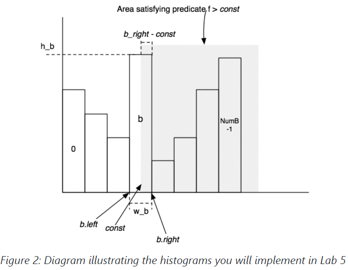
- To estimate the selectivity of a range expression f>const, compute the bucket b that const is in, with width w_b and height h_b. Then, b contains a fraction b_f = h_b / ntups of the total tuples. Assuming tuples are uniformly distributed throughout b, the fraction b_part of b that is > const is (b_right - const) / w_b, where b_right is the right endpoint of b's bucket. Thus, bucket b contributes (b_f x b_part) selectivity to the predicate. In addition, buckets b+1...NumB-1 contribute all of their selectivity (which can be computed using a formula similar to b_f above). Summing the selectivity contributions of all the buckets will yield the overall selectivity of the expression. Figure 2 illustrates this process.
为了估计一个范围表达式f>const的选择性,计算const所在的桶b,其宽度为w_b,高度为h_b。那么,b包含了全部 tuples 中的一部分b_f = h_b / ntups。假设 tuples 均匀地分布在整个b中,b中大于const的部分b_part是(b_right - const)/ w_b,其中b_right是b的桶的右端点。因此,b桶对谓词贡献了(b_f x b_part)的选择性。此外,b+1...NumB-1桶贡献了它们所有的选择性(可以用类似于上面b_f的公式来计算)。将所有桶的选择性贡献相加,将产生表达式的整体选择性。图2说明了这个过程。
- Selectivity of expressions involving less than can be performed similar to the greater than case, looking at buckets down to 0.
涉及小于的表达式的选择性可以类似于大于的情况下进行,看下到0的桶。
In the next two exercises, you will code to perform selectivity estimation of joins and filters.
在接下来的两个练习中,你将用代码来执行连接和过滤器的选择性估计。
# Exercise 1: IntHistogram.java
You will need to implement some way to record table statistics for selectivity estimation. We have provided a skeleton class, IntHistogram that will do this. Our intent is that you calculate histograms using the bucket-based method described above, but you are free to use some other method so long as it provides reasonable selectivity estimates.
你将需要实现一些方法来记录表的统计数据,以便进行选择性估计。我们提供了一个骨架类,IntHistogram,它可以做到这一点。我们的目的是让你使用上面描述的基于桶的方法来计算直方图,但你也可以自由地使用其他方法,只要它能提供合理的选择性估计。
We have provided a class StringHistogram that uses IntHistogram to compute selecitivites for String predicates. You may modify StringHistogram if you want to implement a better estimator, though you should not need to in order to complete this lab.
我们提供了一个StringHistogram类,它使用IntHistogram来计算字符串谓词的选取。如果你想实现一个更好的估计器,你可以修改StringHistogram,尽管你不需要为了完成这个实验而修改。
After completing this exercise, you should be able to pass the IntHistogramTest unit test (you are not required to pass this test if you choose not to implement histogram-based selectivity estimation).
完成这个练习后,你应该能够通过IntHistogramTest单元测试(如果你选择不实现基于直方图的选择性估计,你不需要通过这个测试)。
# Exercise 2: TableStats.java
The class TableStats contains methods that compute the number of tuples and pages in a table and that estimate the selectivity of predicates over the fields of that table. The query parser we have created creates one instance of TableStats per table, and passes these structures into your query optimizer (which you will need in later exercises).
TableStats类包含了计算一个表中 tuples 和页数的方法,以及估计该表字段上的谓词的选择性的方法。我们创建的查询分析器为每个表创建一个TableStats的实例,并将这些结构传递给你的查询优化器(在后面的练习中你会需要它)。
You should fill in the following methods and classes in TableStats:
你应该在TableStats中填写以下方法和类。
Implement the TableStats constructor: Once you have implemented a method for tracking statistics such as histograms, you should implement the TableStats constructor, adding code to scan the table (possibly multiple times) to build the statistics you need.
实现TableStats构造函数。一旦你实现了跟踪统计的方法,如直方图,你应该实现TableStats构造函数,添加代码来扫描表(可能是多次)以建立你需要的统计。
Implement estimateSelectivity(int field, Predicate.Op op, Field constant): Using your statistics (e.g., an IntHistogram or StringHistogram depending on the type of the field), estimate the selectivity of predicate field op constant on the table.
实现 estimateSelectivity(int field, Predicate.Op op, Field constant)。使用你的统计数据(例如,根据字段的类型,使用IntHistogram或StringHistogram),估计predicate字段op常量对表的选择性。
Implement estimateScanCost(): This method estimates the cost of sequentially scanning the file, given that the cost to read a page is costPerPageIO. You can assume that there are no seeks and that no pages are in the buffer pool. This method may use costs or sizes you computed in the constructor.
实现 estimateScanCost()。这个方法估计顺序扫描文件的成本,考虑到读取一个页面的成本是costPerPageIO。你可以假设没有寻道,也没有页面在缓冲池中。这个方法可以使用你在构造函数中计算的成本或大小。
Implement estimateTableCardinality(double selectivityFactor): This method returns the number of tuples in the relation, given that a predicate with selectivity selectivityFactor is applied. This method may use costs or sizes you computed in the constructor.
实现 estimateTableCardinality(double selectivityFactor)。该方法返回关系中 tuples 的数量,考虑到应用了具有选择性的selectivityFactor的谓词。这个方法可以使用你在构造函数中计算的成本或大小。
You may wish to modify the constructor of TableStats.java to, for example, compute histograms over the fields as described above for purposes of selectivity estimation.
你可能希望修改TableStats.java的构造函数,例如,为了选择性估计的目的,计算上述字段的直方图。
After completing these tasks you should be able to pass the unit tests in TableStatsTest.
完成这些任务后,你应该能够通过TableStatsTest的单元测试。
# 2.2.4 Join Cardinality
Finally, observe that the cost for the join plan p above includes expressions of the form joincost((t1 join t2) join t3). To evaluate this expression, you need some way to estimate the size (ntups) of t1 join t2. This join cardinality estimation problem is harder than the filter selectivity estimation problem. In this lab, you aren't required to do anything fancy for this, though one of the optional excercises in Section 2.4 includes a histogram-based method for join selectivity estimation.
最后,观察一下,上面的连接计划p的成本包括形式为joincost((t1 join t2) join t3)的表达。为了评估这个表达式,你需要一些方法来估计t1 join t2的大小(ntups)。这个连接cardinality估计问题比过滤器的选择性估计问题更难。在这个实验中,你不需要为此做任何花哨的事情,尽管第2.4节中的一个可选的练习包括一个基于直方图的连接选择性估计的方法。
While implementing your simple solution, you should keep in mind the following:
在实施你的简单解决方案时,你应该牢记以下几点。
For equality joins, when one of the attributes is a primary key, the number of tuples produced by the join cannot be larger than the cardinality of the non-primary key attribute.
对于等价连接,当其中一个属性是主键时,由连接产生的 tuples 的数量不能大于非主键属性的cardinality。
For equality joins when there is no primary key, it's hard to say much about what the size of the output is -- it could be the size of the product of the cardinalities of the tables (if both tables have the same value for all tuples) -- or it could be 0. It's fine to make up a simple heuristic (say, the size of the larger of the two tables).
对于没有主键的等价连接,很难说输出的大小是什么--它可能是表的cardinalities的乘积的大小(如果两个表的所有 tuples 都有相同的值)--或者它可能是0。
For range scans, it is similarly hard to say anything accurate about sizes. The size of the output should be proportional to the sizes of the inputs. It is fine to assume that a fixed fraction of the cross-product is emitted by range scans (say, 30%). In general, the cost of a range join should be larger than the cost of a non-primary key equality join of two tables of the same size.
对于范围扫描,同样也很难对尺寸说得准确。输出的大小应该与输入的大小成正比。假设交叉产物的一个固定部分是由范围扫描发出的(比如,30%),是可以的。一般来说,范围连接的成本应该大于相同大小的两个表的非主键平等连接的成本。
# Exercise 3: Join Cost Estimation
The class JoinOptimizer.java includes all of the methods for ordering and computing costs of joins. In this exercise, you will write the methods for estimating the selectivity and cost of a join, specifically:
JoinOptimizer.java类包括所有用于排序和计算连接成本的方法。在这个练习中,你将写出用于估计 join 的 selectivity 和 cost 的方法,特别是:
Implement estimateJoinCost(LogicalJoinNode j, int card1, int card2, double cost1, double cost2): This method estimates the cost of join j, given that the left input is of cardinality card1, the right input of cardinality card2, that the cost to scan the left input is cost1, and that the cost to access the right input is card2. You can assume the join is an NL join, and apply the formula mentioned earlier.
实现 estimateJoinCost(LogicalJoinNode j, int card1, int card2, double cost1, double cost2) 。这个方法估计了连接j的成本,考虑到左边的输入是cardinality card1,右边的输入是cardinality card2,扫描左边输入的成本是cost1,访问右边输入的成本是card2。你可以假设这个连接是一个NL连接,并应用前面提到的公式。
Implement estimateJoinCardinality(LogicalJoinNode j, int card1, int card2, boolean t1pkey, boolean t2pkey): This method estimates the number of tuples output by join j, given that the left input is size card1, the right input is size card2, and the flags t1pkey and t2pkey that indicate whether the left and right (respectively) field is unique (a primary key).
实现 estimateJoinCardinality(LogicalJoinNode j, int card1, int card2, boolean t1pkey, boolean t2pkey) 。这个方法估计了j连接输出的 tuples 数,给定左边的输入是大小为card1,右边的输入是大小为card2,以及指示左边和右边(分别)字段是否唯一(主键)的标志t1pkey和t2pkey。
After implementing these methods, you should be able to pass the unit tests estimateJoinCostTest and estimateJoinCardinality in JoinOptimizerTest.java.
实现这些方法后,你应该能够通过JoinOptimizerTest.java中的单元测试 estimateJoinCostTest 和 estimateJoinCardinality。
# 2.3 Join Ordering
Now that you have implemented methods for estimating costs, you will implement the Selinger optimizer. For these methods, joins are expressed as a list of join nodes (e.g., predicates over two tables) as opposed to a list of relations to join as described in class.
现在你已经实现了估计成本的方法,你将实现Selinger优化器。对于这些方法,连接被表达为一个连接节点的列表(例如,对两个表的谓词),而不是课堂上描述的连接关系的列表。
Translating the algorithm given in lecture to the join node list form mentioned above, an outline in pseudocode would be:
将讲座中给出的算法转化为上述的连接节点列表形式,伪代码的概要是:。
1. j = set of join nodes
2. for (i in 1...|j|):
3.     for s in {all length i subsets of j}
4.       bestPlan = {}
5.       for s' in {all length d-1 subsets of s}
6.            subplan = optjoin(s')
7.            plan = best way to join (s-s') to subplan
8.            if (cost(plan) < cost(bestPlan))
9.               bestPlan = plan
10.      optjoin(s) = bestPlan
11. return optjoin(j)
2
3
4
5
6
7
8
9
10
11
To help you implement this algorithm, we have provided several classes and methods to assist you. First, the method enumerateSubsets(List v, int size) in JoinOptimizer.java will return a set of all of the subsets of v of size size. This method is VERY inefficient for large sets; you can earn extra credit by implementing a more efficient enumerator (hint: consider using an in-place generation algorithm and a lazy iterator (or stream) interface to avoid materializing the entire power set).
为了帮助你实现这个算法,我们提供了几个类和方法来帮助你。首先,JoinOptimizer.java中的enumerateSubsets(List v, int size)方法将返回一个大小为v的所有子集的集合。这个方法对于大型集合来说效率非常低;你可以通过实现一个更有效的枚举器来获得额外的分数(提示:考虑使用原地生成算法和懒惰迭代器(或流)接口来避免物化整个幂集)。
Second, we have provided the method:
第二,我们提供了方法。
    private CostCard computeCostAndCardOfSubplan(Map<String, TableStats> stats,
                                                Map<String, Double> filterSelectivities,
                                                LogicalJoinNode joinToRemove,
                                                Set<LogicalJoinNode> joinSet,
                                                double bestCostSoFar,
                                                PlanCache pc)
2
3
4
5
6
Given a subset of joins (joinSet), and a join to remove from this set (joinToRemove), this method computes the best way to join joinToRemove to joinSet - {joinToRemove}. It returns this best method in a CostCard object, which includes the cost, cardinality, and best join ordering (as a list). computeCostAndCardOfSubplan may return null, if no plan can be found (because, for example, there is no left-deep join that is possible), or if the cost of all plans is greater than the bestCostSoFar argument. The method uses a cache of previous joins called pc (optjoin in the psuedocode above) to quickly lookup the fastest way to join joinSet - {joinToRemove}. The other arguments (stats and filterSelectivities) are passed into the orderJoins method that you must implement as a part of Exercise 4, and are explained below. This method essentially performs lines 6--8 of the psuedocode described earlier.
给出一个连接的子集(joinSet),以及一个要从这个子集中移除的连接(joinToRemove),这个方法计算出将joinToRemove连接到joinSet的最佳方法--{joinToRemove}。它在一个CostCard对象中返回这个最佳方法,其中包括成本、cardinality和最佳连接顺序(作为一个列表)。如果找不到计划(因为,例如,没有可能的左深连接),或者如果所有计划的成本都大于bestCostSoFar参数,computeCostAndCardOfSubplan可能返回null。该方法使用了一个叫做pc(上面的psuedocode中的optjoin)的先前连接的缓存来快速查找joinSet的最快方式--{joinToRemove}。其他参数(stats和filterSelectivities)被传递到你必须实现的orderJoins方法中,作为练习4的一部分,下面会有解释。这个方法基本上是执行前面描述的假代码的第6-8行。
Third, we have provided the method:
第三,我们提供了方法。
    private void printJoins(List<LogicalJoinNode> js,
                           PlanCache pc,
                           Map<String, TableStats> stats,
                           Map<String, Double> selectivities)
2
3
4
This method can be used to display a graphical representation of a join plan (when the "explain" flag is set via the "-explain" option to the optimizer, for example).
这种方法可以用来显示连接计划的图形表示(例如,当通过优化器的"-explain "选项设置 "explain "标志时)。
Fourth, we have provided a class PlanCache that can be used to cache the best way to join a subset of the joins considered so far in your implementation of Selinger (an instance of this class is needed to use computeCostAndCardOfSubplan).
第四,我们提供了一个PlanCache类,可以用来缓存到目前为止在你的Selinger实现中所考虑的连接子集的最佳方式(使用computeCostAndCardOfSubplan需要这个类的一个实例)。
# Exercise 4: Join Ordering
In JoinOptimizer.java, implement the method:
在JoinOptimizer.java中,实现这个方法。
  List<LogicalJoinNode> orderJoins(Map<String, TableStats> stats,
                   Map<String, Double> filterSelectivities,
                   boolean explain)
2
3
This method should operate on the joins class member, returning a new List that specifies the order in which joins should be done. Item 0 of this list indicates the left-most, bottom-most join in a left-deep plan. Adjacent joins in the returned list should share at least one field to ensure the plan is left-deep. Here stats is an object that lets you find the TableStats for a given table name that appears in the FROM list of the query. filterSelectivities allows you to find the selectivity of any predicates over a table; it is guaranteed to have one entry per table name in the FROM list. Finally, explain specifies that you should output a representation of the join order for informational purposes.
这个方法应该在joins类成员上操作,返回一个新的List,这个List指定了应该进行的连接的顺序。这个列表中的第0项表示左深计划中最左、最底的连接。返回的列表中相邻的连接应该至少共享一个字段,以确保计划是左深的。这里stats是一个对象,让你找到出现在查询的FROM列表中的给定表名的TableStats。 filterSelectivities让你找到表的任何谓词的选择性;它保证在FROM列表中的每个表名有一个条目。最后,explain指定了你应该输出一个连接顺序的表示,以供参考。
You may wish to use the helper methods and classes described above to assist in your implementation. Roughly, your implementation should follow the psuedocode above, looping through subset sizes, subsets, and sub-plans of subsets, calling computeCostAndCardOfSubplan and building a PlanCache object that stores the minimal-cost way to perform each subset join.
你可能希望使用上面描述的辅助方法和类来帮助你实现。大致上,你的实现应该遵循上面的假设代码,通过子集大小、子集和子集的子计划进行循环,调用computeCostAndCardOfSubplan并建立一个PlanCache对象来存储执行每个子集连接的最小成本方式。
After implementing this method, you should be able to pass all the unit tests in JoinOptimizerTest. You should also pass the system test QueryTest.
实现这个方法后,你应该能够通过JoinOptimizerTest的所有单元测试。你还应该通过系统测试QueryTest。
# 2.4 Extra Credit
In this section, we describe several optional excercises that you may implement for extra credit. These are less well defined than the previous exercises but give you a chance to show off your mastery of query optimization! Please clearly mark which ones you have chosen to complete in your report, and briefly explain your implementation and present your results (benchmark numbers, experience reports, etc.)
在这一节中,我们描述了几个可选的练习,你可以实施这些练习来获得额外的分数。这些练习没有前面的练习那么明确,但可以让你有机会展示你对查询优化的掌握程度 请在你的报告中清楚地标出你选择完成的练习,并简要地解释你的执行情况和介绍你的结果(基准数字、经验报告等)。
Bonus Exercises. Each of these bonuses is worth up to 5% extra credit:
奖励练习。这些奖金中的每一个都价值高达5%的额外信用。
Add code to perform more advanced join cardinality estimation. Rather than using simple heuristics to estimate join cardinality, devise a more sophisticated algorithm.
添加代码以执行更高级的连接心率估计。与其使用简单的启发式方法来估计连接的cardinality,不如设计一个更复杂的算法。
One option is to use joint histograms between every pair of attributes a and b in every pair of tables t1 and t2. The idea is to create buckets of a, and for each bucket A of a, create a histogram of b values that co-occur with a values in A.
一种选择是在每对表t1和t2中的每对属性a和b之间使用联合直方图。这个想法是创建a的桶,对于a的每个桶A,创建一个与A中a值共同出现的b值的直方图。
Another way to estimate the cardinality of a join is to assume that each value in the smaller table has a matching value in the larger table. Then the formula for the join selectivity would be: 1/(Max(num-distinct(t1, column1), num-distinct(t2, column2))). Here, column1 and column2 are the join attributes. The cardinality of the join is then the product of the cardinalities of t1 and t2 times the selectivity.
另一种估计连接的cardinality的方法是假设小表中的每个值在大表中都有一个匹配的值。那么连接选择性的公式将是。1/(Max(num-distinct(t1, column1), num-distinct(t2, column2)))。这里,列1和列2是连接属性。连接的cardinality是t1和t2的cardinality乘以选择性的产物。
Improved subset iterator. Our implementation of enumerateSubsets is quite inefficient, because it creates a large number of Java objects on each invocation.
改进子集迭代器。我们对enumerateSubsets的实现是相当低效的,因为它在每次调用时都会创建大量的Java对象。
In this bonus exercise, you would improve the performance of enumerateSubsets so that your system could perform query optimization on plans with 20 or more joins (currently such plans takes minutes or hours to compute).
在这个奖励练习中,你将提高enumerateSubsets的性能,这样你的系统就可以对有20个或更多连接的计划进行查询优化(目前这样的计划需要几分钟或几小时来计算)。
A cost model that accounts for caching. The methods to estimate scan and join cost do not account for caching in the buffer pool. You should extend the cost model to account for caching effects. This is tricky because multiple joins are running simultaneously due to the iterator model, and so it may be hard to predict how much memory each will have access to using the simple buffer pool we have implemented in previous labs.
一个考虑到缓存的成本模型。估计扫描和连接成本的方法没有考虑到缓冲池中的缓存。你应该扩展成本模型以考虑到缓存效应。这很棘手,因为由于迭代器模型,多个连接是同时运行的,所以可能很难预测使用我们在以前的实验中实现的简单缓冲池,每个人可以获得多少内存。
Improved join algorithms and algorithm selection. Our current cost estimation and join operator selection algorithms (see instantiateJoin() in JoinOptimizer.java) only consider nested loops joins. Extend these methods to use one or more additional join algorithms (for example, some form of in memory hashing using a HashMap).
改进的连接算法和算法选择。我们目前的成本估算和连接运算符选择算法(见JoinOptimizer.java中的instantiateJoin())只考虑嵌套循环的连接。扩展这些方法以使用一个或多个额外的连接算法(例如,使用HashMap的某种形式的内存散列)。
Bushy plans. Improve the provided orderJoins() and other helper methods to generate bushy joins. Our query plan generation and visualization algorithms are perfectly capable of handling bushy plans; for example, if orderJoins() returns the list (t1 join t2 ; t3 join t4 ; t2 join t3), this will correspond to a bushy plan with the (t2 join t3) node at the top.
忙碌的计划。改进所提供的orderJoins()和其他辅助方法,以生成bushy joins。我们的查询计划生成和可视化算法完全能够处理繁忙的计划;例如,如果orderJoins()返回列表(t1 join t2; t3 join t4; t2 join t3),这将对应于一个繁忙的计划,(t2 join t3)节点在顶部。
You have now completed this lab. Good work!
你现在已经完成了这个实验。干得好!
# 3. Logistics
You must submit your code (see below) as well as a short (2 pages, maximum) writeup describing your approach. This writeup should:
你必须提交你的代码(见下文)以及描述你的方法的简短(2页,最多)的文章。这篇报告应该
Describe any design decisions you made, including methods for selectivity estimation, join ordering, as well as any of the bonus exercises you chose to implement and how you implemented them (for each bonus exercise you may submit up to 1 additional page). Discuss and justify any changes you made to the API. Describe any missing or incomplete elements of your code. Describe how long you spent on the lab, and whether there was anything you found particularly difficult or confusing. Description of any extra credit implementation you have done.
描述你所做的任何设计决定,包括选择性估计的方法,连接排序,以及你选择实现的任何奖励练习和你如何实现它们(对于每个奖励练习,你可以提交多达1页的额外内容)。 讨论并证明你对API所作的任何修改。 描述你的代码中任何缺失或不完整的元素。 描述你花了多长时间做这个实验,以及是否有任何你认为特别困难或困惑的地方。 描述你所做的任何额外功劳的实现。
# 3.1. Collaboration
This lab should be manageable for a single person, but if you prefer to work with a partner, this is also OK. Larger groups are not allowed. Please indicate clearly who you worked with, if anyone, on your writeup.
这个实室对一个人来说应该是可以应付的,但如果你喜欢和一个伙伴一起工作,这也是可以的。不允许有较大的团体。如果有的话,请在你的报告中明确指出你和谁一起工作。
# 3.2. Submitting your assignment
We will be using gradescope to autograde all programming assignments. You should have all been invited to the class instance; if not, please let us know and we can help you set up. You may submit your code multiple times before the deadline; we will use the latest version as determined by gradescope. Place the write-up in a file called lab3-writeup.txt with your submission. You also need to explicitly add any other files you create, such as new *.java files.
我们将使用gradescope对所有编程作业进行自动评分。你们应该都被邀请到班级实例中;如果没有,请告诉我们,我们可以帮助你们设置。你可以在截止日期前多次提交你的代码;我们将使用由gradescope确定的最新版本。把写好的东西放在一个叫lab3-writeup.txt的文件里,和你的提交一起。你还需要明确地添加你创建的任何其他文件,如新的*.java文件。
The easiest way to submit to gradescope is with .zip files containing your code. On Linux/MacOS, you can do so by running the following command:
向 gradescope 提交的最简单方法是使用包含你的代码的 .zip 文件。在Linux/MacOS上,你可以通过运行以下命令来实现。
$ zip -r submission.zip src/ lab3-writeup.txt
# 3.3. Submitting a bug
SimpleDB is a relatively complex piece of code. It is very possible you are going to find bugs, inconsistencies, and bad, outdated, or incorrect documentation, etc.
SimpleDB是一个相对复杂的代码。你很可能会发现错误、不一致,以及糟糕的、过时的或不正确的文档等等。
We ask you, therefore, to do this lab with an adventurous mindset. Don't get mad if something is not clear, or even wrong; rather, try to figure it out yourself or send us a friendly email.
因此,我们要求你以一种冒险的心态来做这个实室。如果有不清楚的地方,甚至是错误的地方,不要生气;而是要自己尝试去弄清楚,或者给我们发一封友好的电子邮件。
Please submit (friendly!) bug reports to 6.830-staff@mit.edu. When you do, please try to include:
请提交(友好的!)错误报告到6.830-staff@mit.edu。当你这样做时,请尽量包括。
A description of the bug. A .java file we can drop in the test/simpledb directory, compile, and run. A .txt file with the data that reproduces the bug. We should be able to convert it to a .dat file using HeapFileEncoder. You can also post on the class page on Piazza if you feel you have run into a bug.
一个关于该错误的描述。 一个.java文件,我们可以把它放到test/simpledb目录中,编译并运行。 一个包含再现该错误的数据的.txt文件。我们应该能够用HeapFileEncoder将其转换为.dat文件。 如果你觉得你遇到了一个bug,你也可以在Piazza的类页面上发帖。
# 3.4 Grading
75% of your grade will be based on whether or not your code passes the system test suite we will run over it. These tests will be a superset of the tests we have provided. Before handing in your code, you should make sure it produces no errors (passes all of the tests) from both ant test and ant systemtest.
你的成绩的75%将基于你的代码是否通过我们将对其进行的系统测试套件。这些测试将是我们提供的测试的一个超集。在交出你的代码之前,你应该确保它在ant test和ant systemtest中没有产生错误(通过所有的测试)。
Important: before testing, gradescope will replace your build.xml, HeapFileEncoder.java and the entire contents of the test directory with our version of these files. This means you cannot change the format of .dat files! You should also be careful changing our APIs. You should test that your code compiles the unmodified tests.
重要的是:在测试之前,gradescope 会用我们的版本替换你的 build.xml、HeapFileEncoder.java 以及测试目录中的全部内容。这意味着你不能改变.dat文件的格式! 你也应该小心改变我们的API。你应该测试你的代码是否编译了未修改的测试。
You should get immediate feedback and error outputs for failed tests (if any) from gradescope after submission. The score given will be your grade for the autograded portion of the assignment. An additional 25% of your grade will be based on the quality of your writeup and our subjective evaluation of your code. This part will also be published on gradescope after we finish grading your assignment.
在提交后,你应该从 gradescope 得到即时反馈和失败测试的错误输出(如果有的话)。给出的分数将是你在作业的自动评分部分的成绩。另外25%的分数将基于你的写作质量和我们对你代码的主观评价。在我们给你的作业评分后,这部分也将在 gradescope 上公布。
We had a lot of fun designing this assignment, and we hope you enjoy hacking on it!
我们在设计这项作业时非常有趣,我们希望你能享受到黑客的乐趣!